Score-Based Diffusion Models for Undersampled MRI Reconstruction
BSc thesis · Department of Informatics & Telecommunications, NKUA · PyTorch reimplementation of Song et al., ICLR 2022 (arXiv:2111.08005)
The problem
An MRI scanner does not record an image. It records raw signal in the spatial-frequency domain — k-space — and the image is its 2-D Fourier transform. A full acquisition is slow, which costs money, throughput and patient comfort, and invites motion artefacts. You can make the scan R times faster by keeping only 1/Rof the k-space columns — but then there are fewer measurements than unknowns. The reconstruction is under-determined: infinitely many images fit the data, and the naive answer is a blurry mess. Choosing the right one needs a prior — encoded knowledge of what a brain MRI should look like.
The method — intuition first
Song et al. solved this elegantly. Train one unconditional diffusion model to denoise brain MRI at every noise level; what it really learns is, at any level of corruption, which direction looks “more like a brain”. Generate by running the corruption backwards from pure noise in about a thousand small steps — and steer it with the measurements: before every step, overwrite the k-space columns the scanner actually measured with the real values, so the model only ever invents the columns you skipped. One subtlety makes it work — at each step the working image is deliberately noisy, so the measurement is first corrupted to the current noise level before it is spliced in. Because only the sampling mask changes between acceleration factors, one trained prior serves 4×, 8× and 24× with no retraining, fully unsupervised.
forward   dx = f(x,t) dt + g(t) dw
reverse   dx = [ f(x,t) − g(t)² ∇ₓ log pₜ(x) ] dt + g(t) dw̄
VE-SDE    f = 0,  σ(t) = σ_min (σ_max/σ_min)ᵗ,   σ : 0.01 → 128

data      x̂'ₜ = T⁻¹[ λ·Λ·P⁻¹(Λ)·ŷₜ + (1−λ)·Λ·T·x̂ₜ + (I−Λ)·T·x̂ₜ ]
consist.  λ = 0 → unconditional;  λ = 1 → A x̂'ₜ = ŷₜ exactly
What I reproduced
The authors released only a JAX/Flax implementation. I reimplemented the method in PyTorch: the FFT-based measurement operator, the noised-measurement process, the data-consistency step and all four solver modes, validated by CPU unit tests. Rather than retrain the prior, I converted the authors' pretrained NCSN++ checkpoint from Flax — a name-based remap with per-layer axis transforms — verified across all 473 parameter tensors, loading with zero missing or unexpected keys. On BraTS the reimplementation reproduces the published PSNR/SSIM to within 0.15 dB at every acceleration, for about 2.5 GPU-hours and $1.70 on a spot RTX 4090.
| R | Ours (PSNR / SSIM) | Paper (PSNR / SSIM) | Zero-filled (PSNR / SSIM) |
|---|---|---|---|
| 4× | 40.03 / 0.967 | 39.91 / 0.965 | 28.64 / 0.759 |
| 8× | 37.75 / 0.960 | 37.63 / 0.958 | 26.28 / 0.748 |
| 24× | 29.57 / 0.881 | 29.42 / 0.880 | 20.79 / 0.515 |
The boundary, stated plainly. Reused from the reference score_sde_pytorch port: the NCSN++ architecture, the VE-SDE class and the Predictor–Corrector sampler skeleton. Mine: the measurement operator A = P(Λ)T, the conditioning, the data-consistency step, all four solver modes — and every extension below. The generative prior was pretrained by the original authors; I converted it, and later fine-tuned it. I did not train it from scratch.
What I added
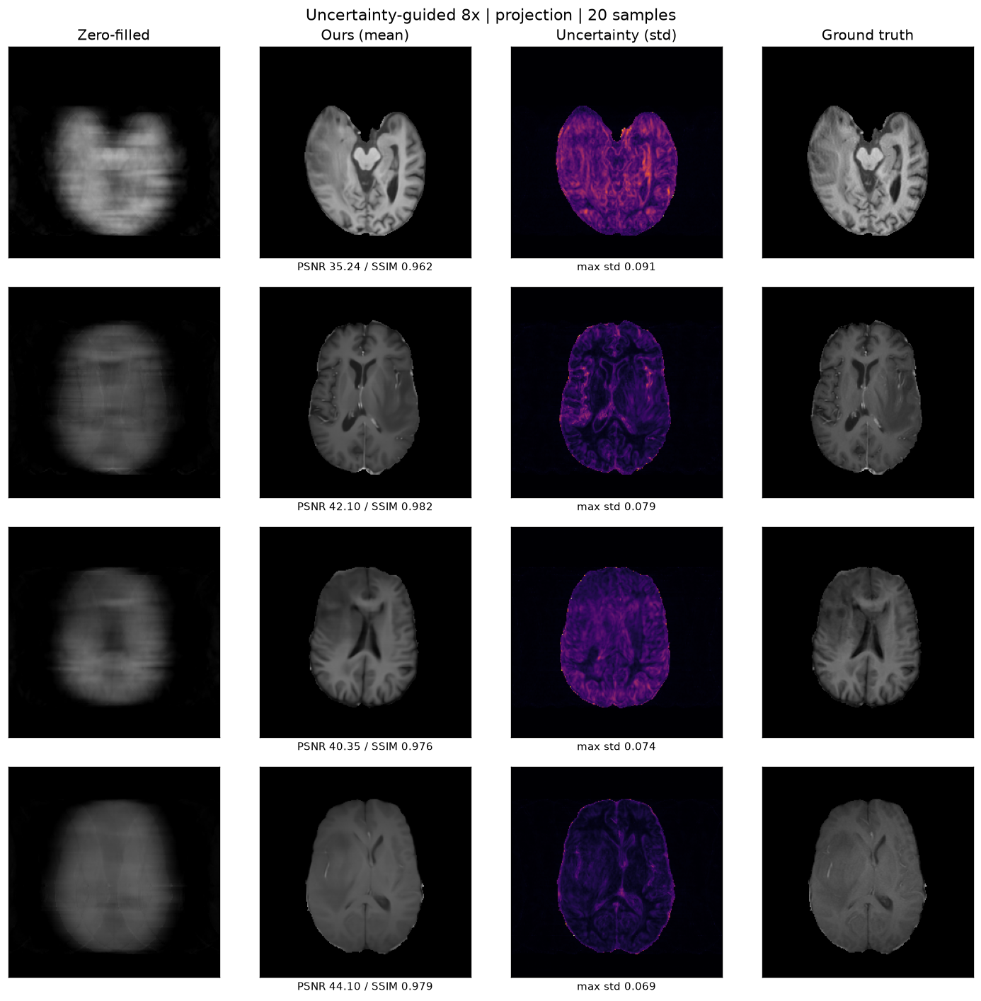
The sampler is stochastic, so I ran it 20 times per scan. The per-pixel mean is an MMSE reconstruction worth +1.4 to +2.0 dB over a single sample; the per-pixel standard deviation is an uncertainty map whose rank correlation with the true error is 0.81–0.87 (Spearman), strengthening as undersampling increases. Cast as a decision rule, deferring the least-reliable half of the pixels cuts the error on the remainder by 27%versus deferring at random. A speed study showed 500 reverse steps match 1000 within 0.3 dB — 2× free, which I then spent on doubling later sample sizes.
Where it breaks, and what fixes it
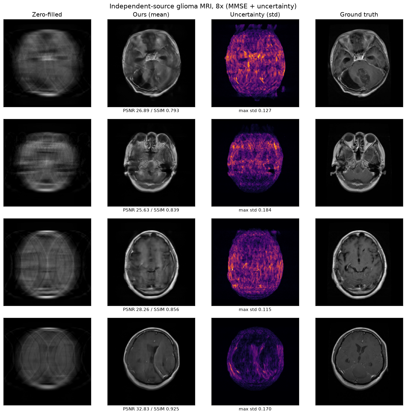
Fed chest CT, the brain prior collapses (37.6 → 19.4 dB) and — the sharper finding — its uncertainty stops being informative (Spearman 0.84 → 0.42): least trustworthy exactly where you would most need it. On real brain MRI from independent hospitals it is not merely worse but actively harmful, scoring below the no-model baseline at 8× and 24×. Pre-specified controls traced the cause to image geometry and scale rather than to the prior. Adapting the model works: 1500 fine-tuning steps on ~40 target-site images — three minutes of A100 time — recover +5.1 / +7.1 / +6.6 dB on 100% of test images, transferring to an unseen source (+8.33 dB, p = 9e-10) with no memorisation signature.
What did not work — two results I kept
The null. Using the uncertainty to choose which frequencies to acquire next ties with random selection (−0.06 ± 0.20 dB SEM, winning 31% of 32 slices). An early 4-slice run had suggested a win; it was noise. It is in the thesis as a null result, because that is what it is.
The bug I documented. My first attempt to constrain the brain support at test time lost 2.1 dB. I blamed the constraint — then a prior-free control proved the constraint was innocent and the bug was mine: I had masked a noisy VE-SDE iterate to zero (where σ_max = 128), handing the score network an off-manifold discontinuity it had never seen. I fixed it, re-ran, and wrote down the correction — because it changed the conclusion. It is the same class of mistake the method itself avoids by noising the measurement, made in a place I did not expect.
Scope & limits
Single-coil, 2-D, magnitude-image MRI with simulated Cartesian undersampling, matching Song et al.; multi-coil, complex-valued and real non-simulated acquisitions are out of scope. There is no clinical validation: PSNR/SSIM are surrogate metrics, and the uncertainty map is a reliability indicator for review, not evidence of diagnostic safety. Counts are images/slices, not patients. The cross-source result is across sources within one public aggregated collection — not a credentialed unseen hospital.
Stack
- PyTorch (+ MPS)
- JAX/Flax checkpoint interop
- NCSN++ / VE-SDE
- Predictor–Corrector sampler
- FFT measurement operators
- piq · NumPy/SciPy stats
- pytest (28 CPU-only tests)
- RunPod · A100 80GB / RTX 4090
- LaTeX (XeLaTeX)